Home linear sweep voltammetry

Linear Potential Sweep Voltammetry - ppt video online download

$ 31.99

4.5

(700)

In stock

Description

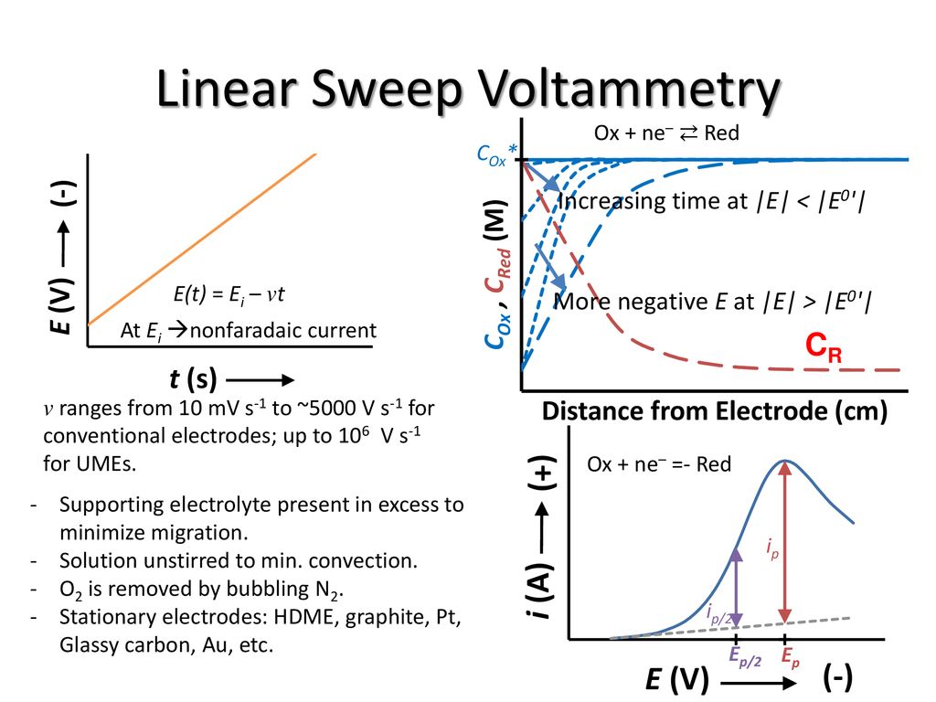
Linear Potential Sweep Voltammetry Ox + ne– ⇄ Red E(t) = Ei – vt At Ei nonfaradaic current v ranges from 10 mV s-1 to ~1000 V s-1 for conventional electrodes; up to 106 V s-1 for UMEs. Supporting electrolyte present in excess to minimize migration. Solution unstirred to min. convection. O2 is removed by bubbling N2. Stationary electrodes: HDME, graphite, Pt, Glassy carbon, Au, etc.
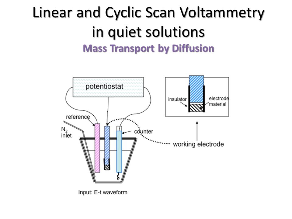
Linear and Cyclic Scan Voltammetry in quiet solutions Mass Transport by Diffusion
Ox + ne– ⇄ Red. E(t) = Ei – vt. At Ei nonfaradaic current. v ranges from 10 mV s-1 to ~1000 V s-1 for conventional electrodes; up to 106 V s-1 for UMEs. Supporting electrolyte present in excess to minimize migration. Solution unstirred to min. convection. O2 is removed by bubbling N2. Stationary electrodes: HDME, graphite, Pt, Glassy carbon, Au, etc.
Ox + ne–  Red. Ox – ne–  Red. reversible electron transfer: DE = |Ep,a – Ep,c| = 59 mV/n. |Ep – Ep/2| = 57 mV/n. ip,a/ip,c = 1. Reversal technique analogous to double-potential step methods. Experiment time scale: 103 s to 10-5 s.
i = n F A CO* (p DO s)1/2 c(s t); c(s t)= numeric function; s t=(nF/RT)(E1-E) s = (nF/RF)n. For reversible electron transfer at 25o C: Randles–Sevčik Eqn (v = scan rate V/s): ip = (2.69 x 105) n3/2 A DO1/2 CO* v1/2. E1/2 = E0’ + (R T) ln(DR/DO)1/2/ (nF) p 1/2c (st) reaches maximum of when n (E – E1/2) is –28.5 mV (Table 6.2.1). ip / (CO* v1/2) = constant (current function) v. Depletion of O near electrode.
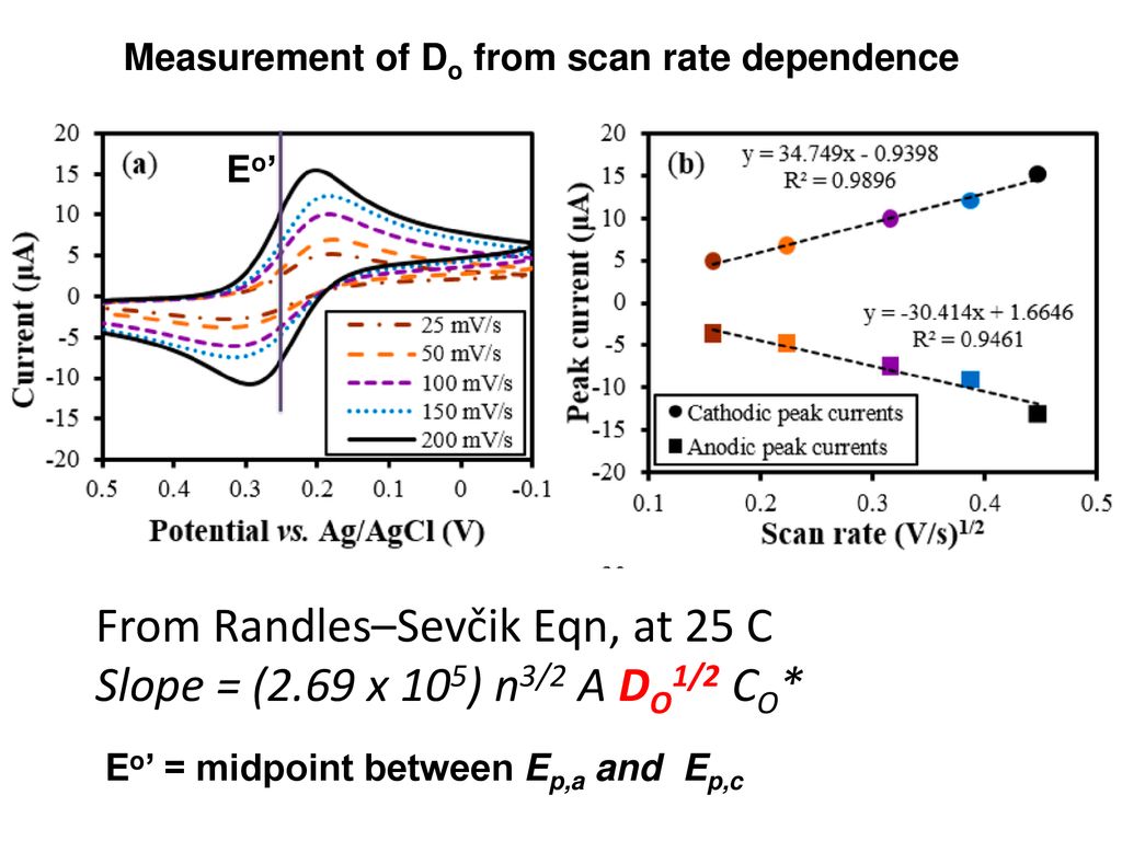
Measurement of Do from scan rate dependence. From Randles–Sevčik Eqn, at 25 C. Slope = (2.69 x 105) n3/2 A DO1/2 CO*
Equal O, R: i ~0.852ip. Recall Cottrell Eqn for E-step (5.2.11): i(t) = n F A DO1/2 CO* / (p t)1/2. Depletion of O near electrode. v. For reversible charge transfer at 25o C: Ep = E1/2 – 28.5/n mV. Ep/2 = E1/ /n mV.
i = n F A CO* (p DO s)1/2 c(s t) + n F A DO CO* f(s t) / r0. i (spherical correction) i (plane) s t = n F v t/(R T) = n F (Ei – E)/(RT) Spherical term dominates if v << R T D / (n F r02) If 0.5 mm radius, D = 10-5 cm2/s, T = 298 K, steady state up to 10 V/s. v.
During potential step experiment (stationary, constant A electrode), charging current disappears after few RuCd (time constant). In potential sweep, ich always flows. Section in B&F. 𝑖 𝑐ℎ =𝑣 𝐶 𝑑 + 𝐸 𝑖 𝑅 𝑠 −𝑣 𝐶 𝑑 𝑒 −𝑡 𝑅 𝑠 𝐶 𝑑. Recall Randles–Sevčik Eqn (6.2.19): ip = (2.69 x 105) n3/2 A DO1/2 CO* v1/2. |idl| = A Cd v below as ich. idl more important at high v. Limit for max useful scan rate and min concentration. |idl| / ip = Cd v1/2 (10-5) / (2.69 n3/2 DO1/2 CO*) Also: EWE = Eapp + iR. x 20. Ru few-hundreds of W ; Cd 10 – 40 mF/cm2. x 40. x 1. v = a. v = 900a. v = 100a.
kf. O + e–  R (Assume semi-inf linear diff, only O initially present, and totally irreversible, one-electron, one-step) i = F A CO* (p DO v)1/2 [(a F) / (R T)]1/2 c(bt) b = a f v. f = F/RT. Compare to Reversible: i = n F A CO* (p DO s)1/2 c(s t) ( a transfer coefficient.
i = F A CO* (p DO v)1/2 [(a F) / (R T)]1/2 c(bt) (6.3.6) One-step, one-electron. For irreversible charge transfer at 25o C: p 1/2c (bt) reaches maximum of (Table 6.3.1). Peak current (6.3.8): ip = (2.99 x 105) n (ana)1/2 A DO1/2 CO* v1/2. Compare to reversible: ip = (2.69 x 105) n3/2 A DO1/2 CO* v1/2. Since ana always < n, ip, irrev smaller than ip, rev. 0 < a < 1. na is the number of electrons involved in the rate-limiting step. Don’t forget: EWE = Eapp + iR. Reversible reaction can appear irreversible if iR drop not compensated! Minimize by using 3-electrode cell, positive feedback compensation at v > 1 V/s, consider UME.
i = n F A CO* (p DO v)1/2 [(a F) / (R T)]1/2 c(bt) (6.3.6) Peak current (6.3.8): ip = (2.99 x 105) n (ana)1/2 A DO1/2 CO* v1/2. Compare to reversible. ip = (2.69 x 105) n3/2 A DO1/2 CO* v1/2. |Ep – Ep/2| = 48/(a na ) mV. 0 < a < 1. Compare to reversible: |Ep – Ep/2| = 57/n mV. Irreversible peak is broader and smaller than reversible peak. As a decreases, peak widens and decreases in magnitude. Unlike reversible, Ep is a function of scan rate for irreversible. Ep shifts more negative for reduction by 30/(a na) m V at 25oC for each 10-fold increase in scan rate.
Irreversible. 48/(a na ) Quasireversible. Between above. Depending on v, a system may show revsible, quasirevsible or irreversible behavior. Appearance of kinetic effects depends on time window of experiment. At small v (long t)  rev, while at large v (short t)  irrev. For n = 1, a = 0.5, T = 25oC, and D = 10-5 cm2/s with L ≈ k0/(39 D v)1/2. Reversible: k0 ≥ 0.3v1/2 cm/s. Quasireversible: 0.3v1/2 cm/s ≥ k0 ≥ 2 x 10-5 v1/2 cm/s. Totally irreversible: k0 ≤ 2 x 10-5 v1/2 cm/s. Increased v makes rxn more difficult (broader wave, shifted negatively for reduction) iR compensation as iR drop distorts linear input ramp of potential sweep. EWE = Eapp + iR.
For reversible electron transfer: DE = |Ep,a – Ep,c| = 59 mV/n. |Ep – Ep/2| = 57 mV/n. ip,a/ip,c = 1. Reversal technique analogous to double-potential step methods. Experiment time scale: 103 s to 10-5 s.
If El is > 35/n mV beyond Ep,c, peak shape generally the same, like forward segment but plotted in opposite direction. Safest to keep El > 90/n mV beyond Ep,c. For reversible electron transfer: ip,a/ip,c = 1. regardless of v and El if El > 35/n mV past Ep,c and D, but must measure ip,a from decaying cathodic current. Also consider: allowing current to decay to nearly zero then performing reverse sweep. Don’t forget charging current: peak must be measured from proper baseline. |ich| = A Cd v. Real experiments: ip measurement imprecise due to uncertainty in correction for charging current, definition of baseline. CV not ideal for quantitative properties reliant on ip (concentration, rate constants), but offers ease of interpreting qual and semi-quan behavior.
If El is > 35/n mV beyond Ep,c, peak shape generally the same, like forward segment but plotted in opposite direction. DEp is a slight function of El, but always close to 59/n mV (25oC). Repeated cycling  steady state (decreased ip,c and increased ip,a) DEp = 58/n mV (25oC).
for quasireversible CV. y (at 25oC) DEp (mV) = kosh/( πDofν)1/2. f = RT/F. Get Ψ from ΔEp, kosh from Ψ. DEp is a function of v, k0, a, and El. Peak separation. If El is 90/n mV beyond peak, El effect is small. 0.3 < a < 0.7, DEp nearly independent of a, mainly depends on y. (Nicholson method) Variation of DEp with v y estimate k0. Beware of uncomp R: ipRu must be small. Effect of Ru most important when currents large and k0  rev limit (DEp only slightly diff from rev value)
Oxid. ΔEp. Theory, working curve. Expt. reducution. Get Ψ from ΔEp, kosh from Ψ. kosh= Ψ( πDofν)1/2; f = RT/F. Model test: kosh is a constant at all ν-values > 65/n mv. R. Nicholson, Anal. Chem. 1965, 37,
Other strategies: Notice i’p must be measured from decaying current of first wave. Assume current decays as t-1/2 to get baseline. Recall Cottrell Eqn for E-step (5.2.11): i(t) = n F A DO1/2 CO* / (p t)1/2. Consider difference between CV and steady-state voltammetry, pulse voltammetry methods.
Mulitstep (O + n1e  R1, then R1 + n2e  R2) similar to two component, but shape depends on DE0 = E20 – E10, reversibility of each step, n1 and n mV < DE0 < 0  single broad wave Ep ind of scan rate. DE0 = 0  single peak with ip between ip(1e), ip(2e) and Ep – Ep/2 = 21 mV. DE0 > 180 mV, 2nd easier than 1st  single wave characteristic of 2e reduction. DE0 = –(2RT/F)ln2 = –35.6 mV (25oC), no interaction between R and O  observed wave has shape of one-e transfer (consider redox polymer with k noninteracting centers: –(2RT/F)ln k) DE0 more positive than –(2RT/F)ln2  2nd e transfer assisted by first.
EC reaction. O + ne ⇄ R. k. R + Z  R-Z (not electroactive) Large k/v. Small k/v. ECcat reaction - catalytic. O + ne ⇄ R. k. R + Z  O + P. Large k/v. Small k/v.
See Wopschall & Shain Anal. Chem. 1967, 39: O + e  R. Osoln. I. Oads. Rsoln. G. Rads. I. Rxn coord. O weakly adsorbed. DG = -nFE. R weakly adsorbed. Adsorption stabilizes species (lower G), otherwise wouldn’t occur spontaneously. V. Post-wave. V. Pre-wave. Osoln. Oads. Rsoln. G. Rads. R strongly adsorbed. O strongly adsorbed. Rxn coord.
Good for qualitative or semi-quantitative description of system based on ip, DEp, recognizable shape, Experimental data - simulation models, obtain k0sh. ip measurement complicated by baseline correction. ich, iR drop, reversal baseline. mathematical corrections, additional experiments. High scan rates: quasireversible , large iR effect. Detection limit ~10-6 to 5x10-7 M; not very sensitive.